The default approach in social science research is to use models which assume a linear relationship between one’s predictor variables and dependent variable. This is due in part to the attractive qualities of OLS linear regression as a modelling technique; particularly its ease of use and interpretability.
Now when it comes to looking at interactions between our independent variables, OLS continues to be the standard approach used. If the relationship between our IV and DV is indeed perfectly linear, then OLS remains a sensible approach. But what about when the relationship is not linear? And how common are truly linear relationships in social science research, anyway?
Nonparametric regression
Nonparametric regression is an alternative modelling approach which is helpful when we are uncertain about the shape of the relationship between our IVs and the DV. When we estimate a standard OLS linear regression, we assume that the functional form for the mean of the outcome is a linear combination of the specified covariates. Nonparametric regression is similar to a standard OLS, but it makes no such assumption.
Instead, nonparametric regression gives us the correct relationship between the outcome and the covariates regardless of their true shape. Using a nonparametric regression is a safe alternative to use in almost all circumstances, because even if the relationship between our IV and DV is truly linear, nonparametric regression results are still consistent (just less efficient…and slow). A further advantage is that we can use the same approach regardless of whether our DV is continuous, ordinal, count or any other level of measurement.
Although nonparametric regression is a way to obtain estimates that are robust to mistakes in specifying the functional form, this robustness comes at a cost. You need many observations and much more time to compute the estimates. Due to the computational intensity, the time it takes to run increases with the number of covariates (see the ‘curse of dimensionality’). So this approach is most useful when you are interested in the relationship between a small number of variables. As computing power increases, and social scientists increasingly run analyses on cloud computing rather than local machines, then the attractiveness of this approach is also likely to increase over the coming years.
Example: Number of Lifetime Sexual Partners
To demonstrate the difference between standard OLS regression interaction effects compared to nonparametric regression, we use data from the National Survey of Sexual Attitudes and Lifestyles (access via UK Data Archive: https://beta.ukdataservice.ac.uk/datacatalogue/series/series?id=2000036).
One of the questions in the survey is the number of sexual partners respondents have had in their lifetime. We might reasonably expect that one important predictor of lifetime sexual partners is a persons age; generally older people will have had more than younger people. We might also expect that the degree to which a person is religious will also be correlated with their number of sexual partners. We might also expect there to be an interaction between these two variables. [FYI: This is me trying to find a fun example, rather than to test a deeply held theory].
In the code below, I open the dataset from the download link above. For simplicity, we will be looking only at males in the survey. I next create a variable for age (in years) and a variable for religious conviction. This is the question: “Importance of Religion and Religious Beliefs Now” (1 = Not Important at All; 4 = Very Important).
Below, we can see the distribution of the total number of partners. We winsorize the variable below to better illustrate the distribution, while analyzing the raw variable in the analyses to come. The number of sexual partners ranges from 0 to 3306 in the raw data, while the top 1% of responses have been constrained to 150 in the below graph.
Next, we can see religious importance broken down. With the majority of people saying that religion is not important to them at all (for international readers, the UK is a very non-religious place).
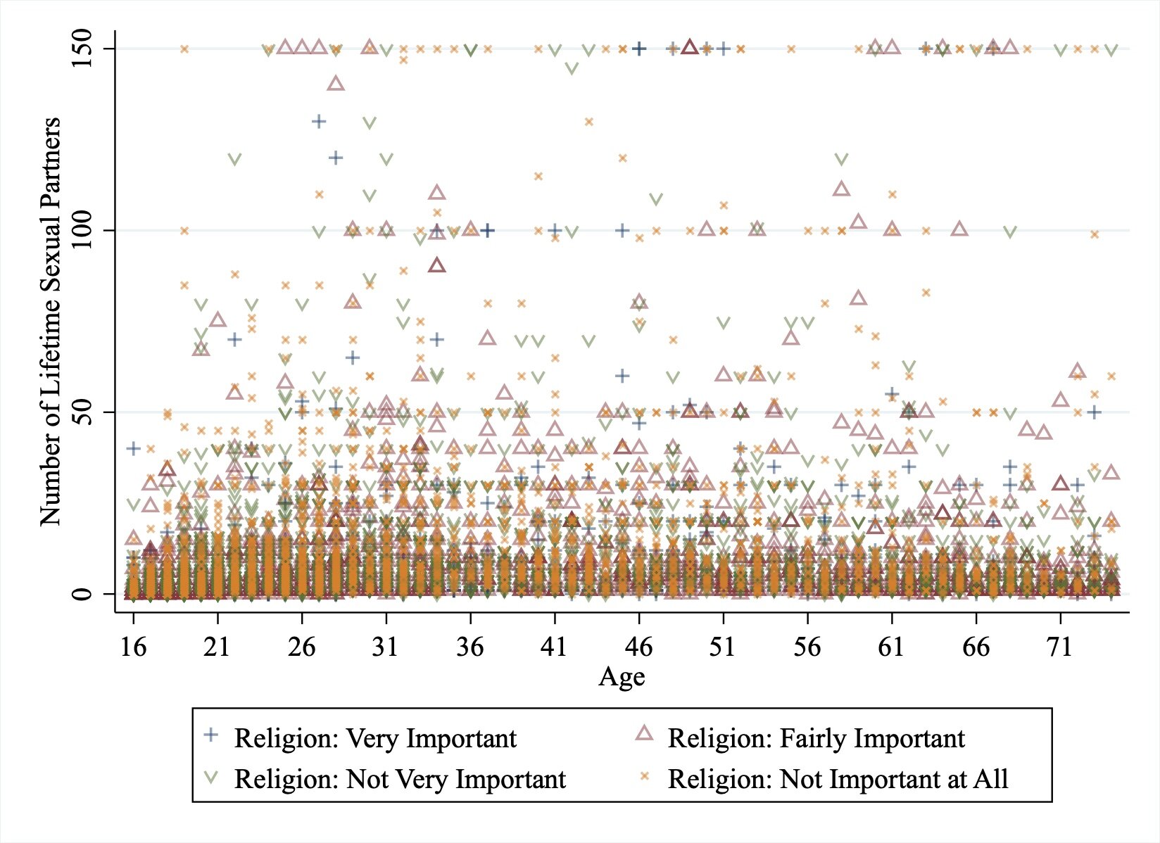
Finally, before we run any models, let’s plot the raw data to see what this looks like. As the below scatter plot shows, there are some extreme outliers, which are likely to have an influential role on our models. In particular, those who report very large numbers of sexual partners (i.e. 1000+) also typically report that religion is not important to them at all.
When we repeat this using a winsorized version of sexual partners (like the histogram above) to limit the extreme outliers, this provides more information on the distribution of responses but this is very messy and difficult to make-out any discernible pattern.
OLS Linear Regression.
We run a boring old OLS linear regression, and include an interaction between age and religious importance. We treat religious importance as a factor variable (basically treating religiosity as four groups), and age as a continuous variable. The interaction results suggest there is a significant difference between some of the religiosity groups in their number of sexual partners across the age spectrum.
To understand the shape of this interaction, we now plot the OLS regression across levels of age and religious importance.
We use the margins command in stata to plot these results.
margins, at(age=(16(5)71) religion_not_important = (1 2 3 4))
marginsplot, recast(line) recastci(rarea) graphregion(color(white))
The results tell a fairly clear story: those who claim religion is not important to them at all report a high number of lifetime sexual partners. This relationship is strongest the older a person is.
Negative Binomial Regression
Now you might be thinking - “Hey there! Number of sexual partners is a count variable, so employing an OLS model it is a poor comparison against this fancy nonparametric regression. Instead we should use a model designed to deal with count variables.” And you’d be right. Next let’s use a negative binomial regression (similar to a Poisson regression model, but for over-dispersed count data).
When we plot the expected number of sexual partners from the negative binomial regression, we see a similar pattern to that found in the OLS regression, except now the relationship between the religious and sexual partners is non-linear.
Nonparametric Regression
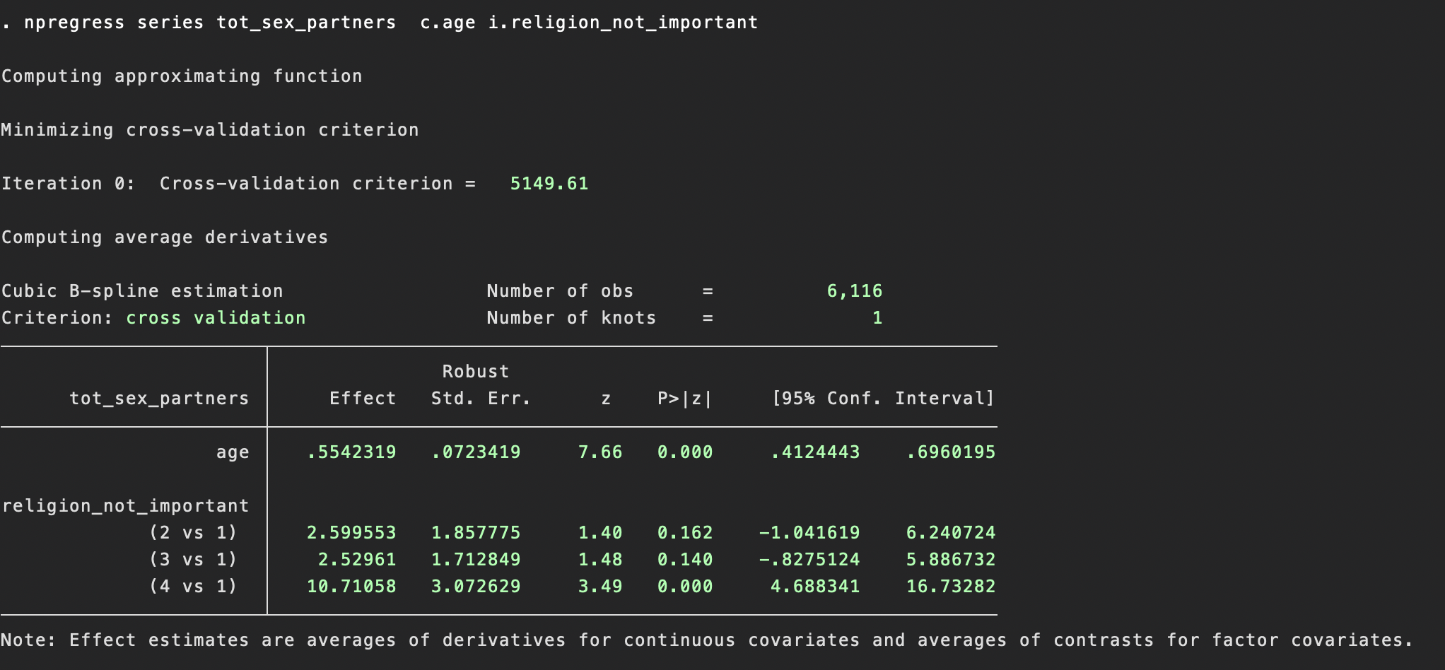
We next model the data as a nonparametric series regression. There are two options here: ‘npregress series’ or ‘npregress kernel’. Stata does a good job of explaining the differences between these approaches in an accessible way here, so I’m going to leave a deeper description of this to another time.
What is clear from the above code and output though is the simplicity of the command. It is simply:
npregress series DV IV1 IV2
Notice that including the interaction in the model is not necessary in nonparametric regression models.
We next use the margins command and marginsplot, just as we would in a normal regression model:
margins religion_not_important, at(age=(16(5)71))
marginsplot, recast(line) recastci(rarea) graphregion(color(white))
Now we see a very different picture emerge. If we focus on young people (e.g., under 30) first, the model predicts that those who were more religious (the blue line) behaved differently compared with other respondents. For those in the most religious group, they had fewer sexual partners when in their late teens and twenties.
The relationship between age and sexual partners is also interesting in later life. With age showing a curvilinear relationship on sexual partners at higher levels of age. Those in the most religious group also show this rise and fall. Keep in mind that this is simply a cross-section of data, and so age is also capturing cohort effects (people who are 60 or 70 now grew up with very different sexual norms than those today, and this may contribute to differences in number of sexual partners).
I do not want to over-interpret the graph, considering that a huge swathe of important variables (e.g., relationship status, values, etc) are not accounted for in the model. My point is simply that the pattern of results is very different using a nonparametric regression, and because we are not imposing linearity on the relationship, the relationship described over is likely to be a better representation of the true relationship found in the world.


